Table of Contents
Introduction
In this study, we will employ some techniques of exploratory data analysis on the RMS Titanic dataset which is made available by Kaggle on its site. The training dataset contains personal and survival information about the passengers of the Titanic.
The analysis will allow us to gain as much insight into the Titanic data. We will uncover the structure of the data to verify underlying assumptions. Some assumptions may reveal interesting insights while others may point towards possible relationships among variables.
Defer cause and effect inferences 
The Titanic dataset presents us with the results of an observational study. The records of the Titanic dataset provides passenger data that have already been observed and recorded. Like most types of observational studies where there is no random assignment and no variables are controlled, it is often very difficult if not impossible to establish causality between variables. However, this exploratory data analysis will allow us, at the minimum, to discover associations and potential predictabilities among the features of the dataset.
Focus on data exploration and data wrangling 
The primary aim of these exercises is to show the features of the python pandas software library that make it a very useful tool in data analysis.
%matplotlib inline
import numpy as np
import pandas as pd
We will be working with the Kaggle Titanic training dataset. After downloading the training data file from Kaggle's website, we then load the data into our workspace and instantiate a pandas dataframe object. Afterwards, we display the first three records from the dataset to verify a successful data load.
CRLF = "\n"
filepath = '..\\Data\\train.csv'
titanic_df = pd.read_csv(filepath)

#Show the first three cases
titanic_df[0:3]
The sample cases show that the Titanic dataset has twelve variables or features: seven variables are of the numeric type (Passengerid, Survived, Pclass, Age, SibSp, Parch and Fare) and four variables are of the character or text type (Name, Sex, Ticket, Cabin and Embarked).
General Properties
Let's use pandas' dataframe info() function to examine the structure of the dataset.
The Titanic training dataset has a 891 observations (each row represents a passenger) and 12 variables (columns).
The dataframe summary also shows that there are rows that contain missing data in three variables (Age, Cabin, and Embarked).
Data Cleaning
Missing Data
Let's determine how much of the missing values make up each of these columns.
print CRLF
print 'Variables and Percent Missing Values'

#Proportion of missing values
(titanic_df.isnull().sum()/len(titanic_df)*100)[(lambda x: x > 0)]
Rows with missing values in the Age column make up about 19.87% of the observations. This missing value rate is quite considerable. Let's display some rows or cases where we find that the Age data is missing.
There does not seem to be pattern about the missingness in the Age variable. We might think that a missing age seems to be paired with a missing cabin data for each passenger. However, there are rows when this isn't so. For our purposes, we will further examine the Age variable later and see if we can consider filling the missing values with imputed values.
Seventy-seven percent of the titanic dataset are missing cabin information. This is a considerable amount, more than three-fourths of the total number of cases. So, we may consider doing a listwise deletion technique on the cabin variable and utilize a complete-case analysis of the other predictor variables when studying their relationship with the response variable (Survived). An idea would be that one may come up with imputed categorical values to fill the missing Cabin information based on a function that interpolates from related features such as the price of the ticket (Fare).
The Embarked variable only had two missing values. We will remember to revert to a pair-wise (available-case analysis) technique when using this feature in our analysis.
Dealing with missing age data
About 19.87% of the cases do not have a value under the Age variable. A less than 5% missing rate is the traditional cutoff when considering whether or not to fill the missing values with computed or imputed data.
Some studies have shown (Schafer 1999) that filling in values where less than 5% of the data is missing completely at random (MCAR) has an insignificant effect on the statistical inferences (especially those that involve variance).
I have decided to try to fill in the missing ages because a preliminary consideration of the missingness of the ages in context with the other variables seems to suggest that they are of a random nature (MCAR).
In the code statements that follow, I will be using a principled missing data method called Multiple Imputation by Chained Equations (MICE) to impute the missing ages.
from fancyimpute import MICE

slice_age_missing = np.asarray(titanic_df[['Age', 'Pclass','Fare']])
imputer = MICE(n_imputations=100, impute_type='col', verbose=False)
slice_age_imputed = imputer.complete(slice_age_missing)
We will do some data transformation by adding a new column called X_Imputed_Age to hold the array of imputed ages that the MICE algorithm generated for us.
Let's take a glimpse of some records which received imputed age values.
I have given the summary statistics below from the original and imputed sets of ages to verify the results of our imputation and determine the difference between their means and the standard deviations.
The measures of central tendency and dispersion seem very close and so we are satisfied with the results of the MICE imputation.
Exploratory Data Analysis
Univariate Data Analysis
In this section, we will focus on discovering information about the data based on a single variable each passenger observation.
Survived
Naturally, the first thing that we'd be curious about from our data is: how many passengers survived and how many died?
We can visualize the extent of the differences between the two groups using the bar plots below.

The Titanic dataset has information on 891 passengers. According to Wikipedia, there were approximately 1,317 passengers in the ship. So we can consider our dataset as a sample of the entire population of passengers in the Titanic.
In this dataset, a little below two-thirds of the passengers perished in the Titanic (the exact proportion is 0.62) - a total of 342 survived and 549 people perished. We will examine these two groups further and examine their makeup as we discuss bivariate relationships later.
Gender
Men comprise about 65% of the total passengers in the Titanic dataset, outnumbering women by a ratio of approximately 2 to 1 (the exact ratio is 1.84). Women make up for about 35% of the passengers.
It is interesting to note that the proportions in the sample closely follows what Wikipedia reported. According to Wikipedia, 869 (66%) of Titanic's approximately 1,317 passengers were male and 447 (34%) were female. This similariity is supports validates the representativeness of our sample.
| Gender | Number of Passengers |
|---|---|
| Male | 577 |
| Female | 314 |
| Total | 891 |

Ticket Class (Pclass)
The Pclass variable holds code that represents the ticket class of a passenger. Generally, the lower the ticket class number, the more expensive the fare.
| Code | Description |
|---|---|
| 1 | First Class |
| 2 | Second Class |
| 3 | Third Class |
How many passengers held first, second or third class tickets? Let's find out.
Most of the passengers held third class tickets (491 tickets which is about 55%) in our sample dataset. This is followed by first class ticket holders (216 tickets which is about 24%) and third second class passengers held 184 of the tickets (which is about 21%).
According to Wikipedia, out of the approximately 1,317 passengers, about 24.6% held first class tickets, 21.5% held second class tickets and 53.8% held third class tickets. This shows that our sample closely follows the makeup of the Titanic population.

Fare
Fare is another variable that did not contain missing values. The price to board this special vessel depends on the accommodations one wants to expect for the trip. Accordingly, the rich paid premium and passengers in the third class cabins still paid a somewhat costly amount.
The table below shows the cost of accommodations in one of Titanic's suites or cabins. This information is taken from an article called "Suites and Cabins for Passengers on the Titanic" by Stephen Spignesi.

Some summary statistics on the Fare variable of the Titanic dataset is shown below.
The typical is 32 British pounds, about enough to get someone a first-class cabin. This mean fare (32.20) is greater than the median (14.45) and so we expect the distribution to be strongly positively skewed. This is confirmed by the histogram and the boxplot below.
There are data points that have zero fare amounts and there are also some with fare amounts in excess of a couple of standard deviations from the typical fare. We will investiget them in the next section.

Outliers — Fare
Let's display the passenger information on some with zero fare amounts.
Let us take a look at Mr. Jonkheer John George Reuchlin (Passenger ID 823). In our sample dataset, Mr. Reuchlin is 38 years old, and had a first class ticket yet he paid 0.0 on his fare. Unfortunately, he did not survive the catastrophe.

According to Encyclopedia Titanica, it turns out that Mr. Reuchlin was carrying a complementary ticket because of his position with the Holland America Line and that he was on the Titanic to evaluate the ship.
Let us know look into those who paid exorbitant fares.
Miss Anna Ward was a personal maid of Mrs. Charlotte Cardeza, daughter of a rich textile entrepreneur. Mr. Thomas Drake Martinez Cardeza is part of the travelling companions of Miss Anna Ward. Mr. Gustave J. Lesurer is the manservant of Mr. Thomas Drake Cardeza. It seems like these passengers are part of the same group of people who all paid expensively for the trip.
Age
Earlier, we have wrangled with the dataset and imputed the missing age values into a new variable which we call X_Imputed_Age. We will now show some descriptive statistics on the imputed ages of the passenger sample data.
Most of the passengers (75%) were 35 years old or younger and half of them were less than 30 years old.

The mean and the median of the imputed ages are very close (29 years) so we can expect a symmetric distribution about the mean. Because the distribution of the ages is nearly normal, we can also infer that 95% of the data would fall within 3 to 55 years. A standard deviation of 13 is explains the very dispersed distribution of passenger ages.
Outliers — Age
Notice that we have a count on ages that are zero or close to zero. Let's investigate this. The code below will display cases where the imputed age value is less than 1.
Master Assad Alexander Thomas is a Lebanese infant who was 5 months and 7 days old when he, his mother and uncle boarded the Titanic in Cherbourg. They were headed Wilkes-Barre, Pennyslvania. The baby survived and was reunited with his mother.
We also notice that the maximum age is 80. The code below will show us all passengers with age greater than 79.
The query returned Mr. Algernon Henry Barkworth as being 80 years of age. However, we discover that this must have been a mistake because the Enclyclopedia Titanica website shows him to have been born on June 4, 1864. This makes Mr. Barkworth to be 47 years old at the time of the accident.
The code below replaces the Age and X_Imputed_Age (columns 5 and 12) variables for Mr. Barkworth's record (Row 530) with the correct age of 47.
Now that we have corrected the age on the outlier record, let's now display the histogram of the imputed age variable.

Derived Column — Survived
As part of our preliminary data wrangling activities, we will apply some data transformation on the Titanic dataset by using the existing Survived values and making them more descriptive (e.g. "Survived", "Died").
We will add this vector of converted values into the same dataset using the apply() function and call the newly created derived column X_Survived.
def convert_survived(survived):
    if survived == 1:
        return 'Survived'
    else:
        return 'Died'

titanic_df['X_Survived'] = titanic_df.Survived.apply(convert_survived)
Multivariate Data Analysis
We will now turn our attention to exploring possible associations between two or more variables or features. Here are a few questions that aim to get some insights from any relationship between two or more features of the Titanic passenger dataset:
How does one's age relate to one's survival? Did more adults survive the accident compared to children?
What is the gender makeup of Titanic passengers who died or survived? Did more women die compared to men?
Did a man who held a first class ticket had a better chance of surviving than a third class passenger woman?
What can the data tell us about women-and-children-first policy?
In this section, we will be working on the multiple features of each observation and show how combinations of such features may tell us interesting things about the Titanic dataset.
How is age associated with survival in the Titanic?
Is a passenger's age in any way associated with survival or death in the Titanic? We might suppose that age might be a factor in confronting the physical demands and efforts in surviving the calamity. On the other end, childhood might also be a contributing factor to one's survival because the passengers might adhere to the women-and-children-first policy that is usually practiced at sea in the face of such emergencies.
Data Transformation - Maturity Level Based on Age
We start with this bivariate analysis by creating a categorical variable which we will call X_Maturity that takes on the values of either "Adult" or "Child" depending on the passenger's recorded (or imputed) age. To do this, we will define a function called convert_maturity() that returns a descriptive category based on the age parameter that is passed to it.
We will suppose and define a "child" to be anyone below the age of 15 years.
def convert_maturity(age):
    if age >= 15:
        return 'Adult'
    else:
        return 'Child'
We use Pandas' apply() function along with our user-defined convert_maturity function to generate the needed X_Maturity data across all the cases. The resulting vector or series data is then appended as a new column (X_Maturity) in our existing dataset.
Row-wise vectorized operation
Since we are using a Pandas DataFrame, we demonstrate the use of Pandas built-inapply()function along with a user-defined function to execute a vectorized operation on the entire set of observations in the dataset. This makes for a more concise, readable code as well as eliminates the use of loop operations.
titanic_df['X_Maturity'] = titanic_df.X_Imputed_Age.apply(convert_maturity)
Let's take a glimpse of our dataset after adding the new X_Maturity column. The introduction of the X_Maturity column allows us to create subsets of the passenger dataset and extract additional insights based on these groups.
titanic_df.head(5)[['PassengerId','Survived','Name','Sex','Age','X_Imputed_Age','X_Maturity']]
Comparing Deaths Among Children and Adults
Children make up around 13% of the 891 passengers in our Titanic dataset. The rest, or about 87%, are 18 years old or older. The code below and the contingency table that follows show how much within these two groups are those who died and those who survived the accident.
| Survivors | Deaths | Total | Pct Died | |
|---|---|---|---|---|
| Adult | 297 | 516 | 813 | 63 |
| Child | 45 | 33 | 78 | 42 |
| Total | 342 | 549 | 891 | 62 |
A little less than half or 42% of the children who boarded the Titanic perished. However, this is remarkably lower than the number of adults who perished as the dataset informs us that almost 2 out of 3 adult passengers (63%) died.
The bar plots below compare the number of passengers who died and who survived within these two groups (children and adults).

To get a better feel of the comparison between the deaths within these two groups, we can put them in equal footing. We can standardize the counts of deaths and surivors among the children and adult groups by calculating the proportion of deaths between each group.
In the code that follows, we first calculate the proportion of deaths and surivors from within the group of children and then do the same about the deaths and survivors from within the group of adults.
We display the results afterwards in a side-by-side stacked bar plot which is a good tool to visualize these bivariate categorical variables (age/maturity level and survived).

The categorical stacked bar plot above tells us that more adults died within their group than those who perished within the children's group.
Our sample data tells us that 4 out of 10 children died while 6 out of 10 adults perished.
How is gender associated with survival in the Titanic?
What is the gender makeup of Titanic passengers who died or survived? Did more women die compared to men?
In our previous univariate analysis of the gender variable in the Titanic dataset, we know that men outnumber women, but how was a passenger's gender associated to surviving the catastrophe?
To get started, let's tally the number of people who survived and perished and further group them by their gender.
male_victims   = titanic_df[titanic_df.Sex == 'male'].Survived.value_counts()[0]
male_survivors = titanic_df[titanic_df.Sex == 'male'].Survived.value_counts()[1]

female_victims   = titanic_df[titanic_df.Sex == 'female'].Survived.value_counts()[0]
female_survivors = titanic_df[titanic_df.Sex == 'female'].Survived.value_counts()[1]

print CRLF
print 'Male Deaths: {:>14}'.format(male_victims)
print 'Male Survivors: {:>11}'.format(male_survivors)
print CRLF
print 'Female Deaths: {:>12}'.format(female_victims)
print 'Female Survivors: {:>9}'.format(female_survivors)
| Survived | Died | Total | Pct Survived | |
|---|---|---|---|---|
| Male | 109 | 468 | 577 | 19 |
| Female | 233 | 81 | 314 | 74 |
| Total | 342 | 549 | 891 | 38 |
It seems that while there are many male passengers, 8 out of 10 of them did not survive the accident. On the other hand, 1 out of 4 women did not survive the catastrophe.

The number of men who died outnumbered the number of women who died by a factor of 6 (5.78 to be exact). On the other hand, women who survived outnumbered men who survived by a factor of 2.
Ticket Class, Gender and Survival
Did a man who held a first class ticket had a better chance of surviving than a third class passenger woman?
To help us answer this question, we first introduce a derived column called X_Class which consists of the equivalent text description (e.g. First, Second, and Third) of the Pclass value for each row.
def convert_class(Pclass):
    if Pclass == 1:
        return 'First'
    if Pclass == 2:
        return 'Second'
    if Pclass == 3:
        return 'Third'
    else:
        return 'None'

titanic_df['X_Class'] = titanic_df.Pclass.apply(convert_class)
Let's display our newly created derived column.
titanic_df[['PassengerId','Name','Sex', 'Survived','Pclass','X_Class']][:7]
Now that we have a way of descriptively identifying each passenger's ticket class, we can construct and display a contingency table using the pandas crosstab() function. The table allows us to determine the total number of passengers who survived or died within each group of ticket class.
import pandas as pd
pd.crosstab([titanic_df.Sex, titanic_df.X_Class], titanic_df.X_Survived, margins=True)
Among the women, there were more first class passengers (91) who survived than third class women passengers (72). Note that this number of first class women survivors was a little more than twice the number of first class male passengers (45).
It is also noteworthy that seventy-two third class passenger women died. This number is 23% of the total number of women passengers in our dataset; 89% of the total number of women who died, and it is also 8 times the combined number of first and second class women passengers.
There were 72 third class women passengers who survived, half of the total number of third class women passengers in the Titanic dataset. This group also makes up for 8% (72/891) of the total number of Titanic passengers in our dataset. On the other hand, there were 45 first class male passengers who survived, which is 5% (45/891) of the total number of Titanic passengers.
So, to answer our question, a gentleman who held a first class ticket did not have a better chance of surviving than a third class female passenger. Although we should point out that the difference of odds (3%) is slightly low.
Let's now turn our attention to the male passenger group. The number of third class male casualties is quite remarkable. At 300 deaths, it makes up for 64% of the total male deaths across all ticket class.
It might be reasonable to think that first and second class passengers might have received preferential treatment when it came to receiving help. What does the data tell us?
The contingency table below breaks down the passenger frequencies for each passenger class, further classifying them into the number of deaths and survivors within each group. We also include a derived column, Pct. Survived which shows the proportion of passengers who survived within each group.
| Class | Died | Survived | Total | Pct. Survived |
|---|---|---|---|---|
| First | 77 | 45 | 122 | 36.89 |
| Second | 91 | 17 | 108 | 15.74 |
| Third | 300 | 47 | 347 | 13.54 |
| Total | 468 | 109 | 577 |
From the table above, we can see how the proportion of survivors decreases along with the quality of the ticket class (First class being the highest quality and the Third class being the lowest quality). Also, the percentage of first class male passengers who survived within their group (36.89%) were much higher than that of the third class male passenger group (13.54%). The survival rate among first class men were higher than the survival rate among second class men. And the survival rate among second class men were higher than the survival rate among third class men.
The survival rate within passenger ticket class decreases along with the ticket class quality. The data tells us that social status or privilege is associated with survival in the Titanic disaster.
Moreover, if we combine the first class and second class male passenger group's survival rate which is the ratio of the total number of first and second class male passengers who survived over the total number of first and second class male passengers, we will get a survival rate of 26.96%. This survival rate is twice the survival rate of third class male passengers (13.54%).
Perhaps a data visualization through a point plot will assist us in gathering any insight as to the relationship between the two predictor variables (Gender and Passenger Class) and the response variable (Survived).

The point plot above clearly shows that the data indicates that women overall had a better survival rate in the Titanic as did men, regardless of passenger ticket class. Female passengers holding third class tickets even fared better than the affluent male passengers who held first class tickets.
The positive sloping lines indicate a higher comparative survival rate among females against the males belonging to the same passenger class group.
Women and Children First
It is curious to know whether the data provides any evidence that the women and children first policy was adhered to during the sinking of the Titanic.
According to Wikipedia, "women and children first" is a "code of conduct dating from 1852 whereby the lives of women and children were to be saved first in a life-threatening situation".
To help us explore this, we need to perform some data transformation tasks on our current Titanic training dataset and introduce a new derived column called X_Person that will contain information that describes whether the current row or observation is a Man, a Woman or a Child.
Again, we use the pandas dataframe's apply() function to execute our user-defined convert_to_person() function over each row of the dataset to determine the appropriate values for our new variable.
def convert_to_person(row):
    if row['Sex'] == 'male' and row['X_Imputed_Age'] >= 15:
        return 'Man'
    if row['Sex'] == 'female' and row['X_Imputed_Age'] >= 15:
        return 'Woman'
    else:
        return 'Child'

titanic_df.apply(convert_to_person, axis=1)
titanic_df['X_Person'] = titanic_df.apply(convert_to_person, axis=1)
Let's display some records after creating the new X_Person field.
titanic_df[0:10][['PassengerId','Name','Survived','Sex','X_Imputed_Age', 'X_Person']]
Now that we have transformed the table and added the derived column, we can construct a contingency table (below) using the pandas crosstab() function to give us passenger counts of the men, women, and children who survived and perished. We go on further and also group them by their respective passenger classes to give us more insights.
import pandas as pd
pd.crosstab([titanic_df.X_Person, titanic_df.X_Class], titanic_df.X_Survived, margins=True)
At first glance, we can quickly see that women and children managed to get better numbers under the survived column compared to the men. In fact, across almost all passenger classes except in the third class, there were more women and children who survived than died. The number of third class women passengers who survived were just slightly above those among them who died.
Women and children who had first and second class passenger tickets had a remarkable survival chance. Out of 5 children in the first class group, all but one survived (80% survival rate). And no chldren perished in the second class group (100% survival rate).
Only 2 people out of 92 (98% survival rate) women who held first class passenger tickets died and only 6 out of the 66 women who held second class passenger tickets died (91% survival rate).
In remarkable contrast, it is worth noting that almost all men who held second class tickets perished. The mortality rate for this group is 92%. It is probably no coincidence that women and children in the second class group had very high survival rates (91% and 100% respectively) perhaps because of the valiant men who made the ultimate sacrifice.
The seaborn factorplot function will help us visualize the multivariate relationships present in the rates of survival among men, women and children within each passenger class.

The survival rate is determined by getting the ratio of the number of survivors to the number of deaths within each person group (men, women and children). For example, there were 19 children who survived who also held second class tickets. Since none of the children in this group perished, 19/19 makes for a 100% survival rate.
The survival rates of women and children across all passenger classes were consistently high. In fact, they are higher than the survival rates for men across all passenger classes. This provides a strong argument in favor of the notion that the policy of prioritizing the lives of women and children was adhered to during this particular crisis at sea.
The primary aim of this study is to highlight the use of the Python Pandas library and showcase its built-in tools that assist in data wrangling, data transformation, data analysis as well as data visualization. That is what we have done in the preceding sections.
But I would like to pursue this further and employ some techniques of statistical analysis to gain more insight about the data through formal statistical inference.
We will compare the average passenger fare of those who survived with the average passenger fare of those who died in the historic Titanic accident that happened on April 15, 1912.
DATA PREPARATION
Let's tidy up the data to make it ready for the analyses and visualization that we will be doing later on.
From our main Titanic training dataset (titanic_df), we create a subset comprised of passenger fare and survival information from rows whose passenger fare amounts are within three standard deviations from the mean of each group. We also append a column called Outcome to label each row and help identify to which survival group it belongs (Survived or Died).
To ensure independence within a dataset, the sample size should be less than 10% of the population. Thus, we further subset each group and acquire a random sample consisting of 8% of the original group size to ensure independence within the sample.
import pandas as pd

# subset of passengers who survived
t1_survived = titanic_df[(titanic_df.Survived == 1)]

# trim subset to within 3 standard deviations
t1_survived = t1_survived[np.abs(t1_survived.Fare - t1_survived.Fare.mean()) <= (3*t1_survived.Fare.std())].Fare

# convert to a dataframe
t1_survived = t1_survived.to_frame(name="Fare")

# add a column describing each record
t1_survived['Outcome'] = "Survived"

# randomly get 8% of the rows to ensure independence
t1_survived = t1_survived.sample(frac=0.08, random_state=127)

# subset of passengers who died
t1_died = titanic_df[(titanic_df.Survived == 0)]

# trim subset to within 3 standard deviations
t1_died = t1_died[np.abs(t1_died.Fare - t1_died.Fare.mean()) <= (3*t1_died.Fare.std())].Fare

# convert to a dataframe
t1_died = t1_died.to_frame(name="Fare")

# add a column describing each record
t1_died['Outcome'] = "Died"

# randomly get 8% of the rows to ensure independence
t1_died = t1_died.sample(frac=0.08, random_state=127)

frames = [t1_survived, t1_died]
fare_survived_df = pd.concat(frames)
Displayed below is a sample of 5 observations from our newly created fare_survived_df dataframe.
# randomly select 10 records
fare_survived_df.sample(n=5, random_state=127)
Our sample dataset consists of 70 passengers, 27 of whom survived the accident and 43 died. Each passenger or case also brings information about the passenger fare in British pounds.
The statistical summaries of passenger fares for the two groups (Survived and Died) are shown below. The average passenger fare for surviving passengers was 56.04 quids compared to 20.65 quids for the non-surviving group.
Since the mean passenger fare of the Survived group is higher than its median, we can expect a positively skewed distribution for this group. Similarly, the distribution of the passenger fare of the Died group is positively skewed.
The standard deviation of the Survived group is 53.94. The high standard deviation tells us that the passenger fare for the surviving group is more spread out than the passenger fare of the non-surviving group which has a standard deviation of 21.18.
print CRLF
print("Summary of Passenger Fare - Survived:")
print(fare_survived_df[fare_survived_df.Outcome == "Survived"].Fare.describe())
print CRLF
print("Summary of Passenger Fare - Died:")
print(fare_survived_df[fare_survived_df.Outcome == "Died"].Fare.describe())
A comparison of the distribution of the passenger fares for both the surviving and non-surviving passengers is depicted in the boxplots below. We should be reminded that these boxplots represent data that is within three standard deviations of the mean for each group when we prepared the dataset previously. This is done to minimize the amount of outliers which do not significantly affect our findings.

The distribution of passenger fare among the passengers who survived exhibits a strong positive skew. The median passenger fare for this surviving group is 30 British pounds, which is triple the median passenger cost for the non-surviving group (10.46 British pounds).
We can also see that the spread of the passenger fare for the surviving group is more dispersed especially above the 50th and 75th quartile. On the other hand, the length of the middle portion of the boxplot for the non-surviving group is shorter (IQR of 15.34 as opposed to an IQR of 61.50 for the surviving group) which indicates a narrower spread of passenger costs. The passenger cost for this latter group tend to cluster around the mean, affirming its role as a stronger point estimate for average passenger fare of non-survivors.
Another way of assisting us in appreciating the relationship between passenger fare and survival is given in the swarmplot below.

Notice that the red dot markers representing the dead passengers were quite clustered in the lower passenger cost levels. As the passenger fare cost increases, the sparser the number of red dots that appear.
Suppose we want to estimate how much more or less is the difference between the passenger fare of the passengers who survived compared to the passenger fare of those who died in the Titanic accident. We would use a confidence interval for this.
Let's display the summary statistics of our dataset once again:
| Outcome | Mean | Std Dev | n |
|---|---|---|---|
| Survived | 56.04 | 53.94 | 27 |
| Died | 20.65 | 21.18 | 43 |
Confidence interval for the difference between two sample means
Estimating a population parameter such as the difference between two independent groups entails a confidence interval which is of the form:
\begin{equation*} point \mspace{5mu} estimate \mspace{5mu} \pm \mspace{5mu} margin \mspace{5mu} of \mspace{5mu} error \end{equation*}
Since we are interested in the confidence interval on the difference between two sample averages, we use the following form of the confidence interval:
\begin{equation*} (\bar{x}_{survived} - \bar{x}_{died}) \mspace{5mu} \pm \mspace{5mu} t_{df}^* \mspace{5mu} SE \end{equation*}
The margin of error can be calculated as a critical value multiplied by the standard error.
The standard error can be calculated as the square root of the sum of the variances for each group divided by their respective sample sizes.
\begin{equation*} SE_{(\bar{x_1} - \bar{x_2})} = \sqrt{\frac{s_1^2}{n_1} + \frac{s_2^2}{n_2}} \end{equation*}
\begin{equation*} SE_{(\bar{x_1} - \bar{x_2})} = \sqrt{\frac{53.94^2}{27} + \frac{21.18^2}{43}} \end{equation*}
\begin{equation*} SE_{(\bar{x_1} - \bar{x_2})} = 10.87 \end{equation*}
The standard error is 10.87 and this represents an estimate of the standard deviation of the sampling distribution of the difference between the independent sample means of the passenger fares.
The critical t-score can be determined using the degrees of freedom associated with the t-distribution that we need to use for these data.
\begin{equation*} df = min(n_1 - 1, n_2 - 1) \end{equation*}
The degrees of freedom is the lesser sample size between our two groups which is 27 (Survived). We subtract 1 from this lesser value to get the degrees of freedom that we will use which is 26.
The next step is to find the critical t-score. There are a variety of ways to find the critical t-score (e.g. using a t-table). We use the degrees of freedom we just obtained (26) along with the corresponding tail area probability for our desired confidence level. Our desired confidence level in this case will be 95% and we need to find the tail area probability for this desired confidence level. The tail area probability for a two-tailed test sums up to 5% so the upper and lower tail area are 2.5% or 0.025 because of the symmetric characteristic of the t-distribution.
The critical t-score for the upper and lower tail area of 0.025 and a degrees of freedom of 26 can be determined using the stats.t.ppf() function shown below.
import numpy as np
import pandas as pd
import scipy.stats as stats
import matplotlib.pyplot as plt
import math

# get the critical t-score
stats.t.ppf(q=0.025, df=26)
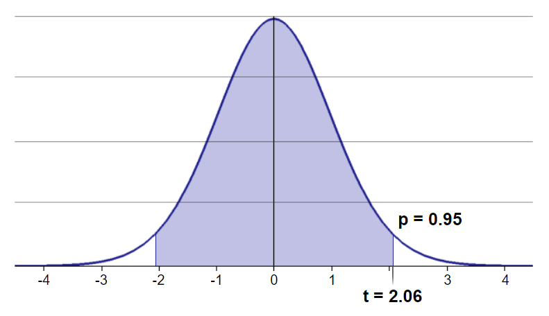
The critical t-score is approximately -2.06. We always use a positive critical value so our final critical t-score is 2.06.
Shown in the visualization below is the confidence level which is the middle symmetric, shaded area in the center of the t-distribution curve and it extends from -2.06 to 2.06. Again, this middle area represents a confidence level of 95% of the sampling distribution of the difference between the sample means.
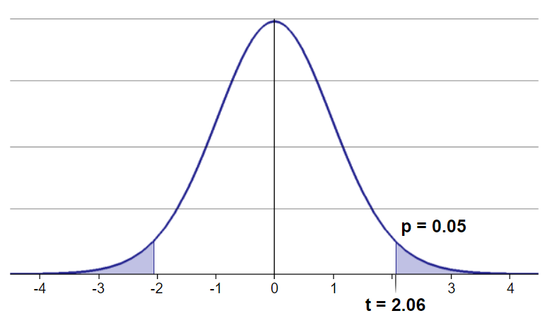
It also shows the critical region (under the context of a 5% significance level) representing the probability of obtaining a sample with a mean passenger fare difference that is as extreme as our observed difference of means between the two passenger groups given that the typical difference of the averages between the two groups is 0.
The two-tailed test displays the critical region which is the unshaded area beyond the critical t-score of 2.06 on the right side fo the curve and less than -2.06 on the left side of the curve.
The margin of error ($margin \mspace{5mu} of \mspace{5mu} error \mspace{5mu} = \mspace{5mu} \mspace{5mu} t_{df}^* \mspace{5mu} SE$) is 22.39 which represents the product of the critical t-score of 2.06 multiplied by the standard error of 10.87.
Conditions for inference for comparing two independent means
There are conditions that we have to meet in order to use our inferential methods. One of these conditions is that there should be independence within each group. We can verify independence within the group with how we used random sampling without replacement and how we only took less than 10% of the population in composing each group. Both n1 and n2 were less than 10% of their respective populations. Since we have made both of these preparations, we can assume that the observations in our study are independent of each other with respect to the response variable (survival) that we are studying. Another condition is that the groups themselves should be independent of each other. There is no pairing going on between each observation across the two groups so we can assume that each group is independent.
The second of these conditions is about the sample size and skew. We took a fair amount of observations for each group and the ample sample sizes should be able to compensate for the skewness in their respective populations.
We finally have all our building blocks and we can now construct the confidence interval for the difference in the means of passenger fares between survivors and non-survivors. It can be estimated using our point estimate, our critical value or critical t-score and our standard error.
| $\bar{x}_{survived}$ | 56.04 |
| $\bar{x}_{died}$ | 20.65 |
| Critical value | 2.06 |
| Standard error | 10.87 |
We use the values we have gathered above to compute the confidence interval at the 95% confidence level.
\begin{equation*} confidence \mspace{5mu} interval \mspace{5mu} = \mspace{5mu} (\bar{x}_{survived} - \bar{x}_{died}) \mspace{5mu} \pm \mspace{5mu} t_{df}^* \mspace{5mu} SE \end{equation*}
\begin{equation*} (56.04 - 20.65) \mspace{5mu} \pm \mspace{5mu} (2.06)(10.87) \end{equation*}
\begin{equation*} 35.39 \mspace{5mu} \pm \mspace{5mu} 22.39 \end{equation*}
\begin{equation*} confidence \mspace{5mu} interval \mspace{5mu} = \mspace{5mu} (13, 57.78) \end{equation*}
Therefore, we are 95% confident that the passenger fares of those who survived the Titanic accident was 13 to 57.78 British pounds more than that paid by those who died.
A difference this high between our samples seems to suggest that there is something going on with the data.
Next, we will work on a hypothesis test for evaluating whether these data provide convincing evidence of a difference in the average passenger fare between those who survived and those who perished in the Titanic accident.
Hypothesis Test — Inference for comparing two independent means
We recall that we would like to evaluate the relationship between passenger fare cost and passenger survival in the Titanic accident.
We prepared a subset of the training data leaving only the survival outcome and the passenger fare costs. There is a total of 874 observations in our dataframe, 335 of the passengers survived and the mean passenger fare for those who survived is 41.68 British pounds. There were 539 passengers who died and the mean passenger fare for those who did not survive is 18.77 British pounds.
Once again, we display the brief summary statistics of our dataset below.
| Outcome | Mean | Std Dev | n |
|---|---|---|---|
| Survived | 56.04 | 53.94 | 27 |
| Died | 20.65 | 21.18 | 43 |
Do our data provide convincing evidence of a difference between the average passenger fares of those who survived and those who died in the Titanic accident?
When doing a hypothesis test, the first step is always to set our hypotheses. The null hypothesis tells us that there is absolutely nothing going on between passenger fares and the survival outcome in the Titanic accident. We can phrase this as the difference of the average passenger fares between survivors and non-survivors is 0. Another way of thinking about this is that the two $\mu$'s from the two populations (survivors and non-survivors)are equal to each other.
The alternative hypothesis is akin to saying that there is something going on between the passenger fares and survival: there is a difference between the two population means or that the difference is not 0.
\begin{equation*} H_0: \mu_{survived} - \mu_{died} = 0 \end{equation*} \begin{equation*} H_A: \mu_{survived} - \mu_{died} \neq 0 \end{equation*}
Calculate our test statistic which is our t-score with 26 degrees of freedom as the observed difference being our point estimate or 35.39 to which we subtract our null value of zero divided by our standard error which we calculated earlier (10.87).
\begin{equation*} T_{df=26} = \frac{35.39 - 0}{10.87} = 3.2557 \end{equation*}
This yields a t-statistic of 3.26.
We must then sketch the sampling distribution before finding the p-value. We need to do this before making a decision on our hypotheses. We shade the tail areas corresponding to our p-value.
We started with a study where we took samples of passengers from two categorical groups of surviving and non-surviving passengers and compared their average passenger fares. Our confidence interval and sample statistics tells us that passengers from the surviving group paid a higher fare on average. However, just because we observed a difference in the sample means does not necessarily mean that there is something going on that is statistically significant in the actual populations.
Thus, we use statistical inference tools to evaluate if this apparent relationship between passenger fare and passenger survival provide evidence of a real difference at the population level.
Note that our data came from an observational study and that we don't have a randomized control group. So that if we do indeed find a significant result, we cannot infer a causal relationship between the independent and response variables.
We use our grouped pandas dataframes as arguments to the stats.ttest_ind() function to obtain the p-value. The same function also provides us with the t-statistic which we also obtained earlier.
import numpy as np
import pandas as pd
import scipy.stats as stats
import matplotlib.pyplot as plt
import math

stats.ttest_ind(a=fare_survived_df[fare_survived_df.Outcome == "Survived"].Fare,
                b=fare_survived_df[fare_survived_df.Outcome == "Died"].Fare,
                equal_var=False)
To recap, the confidence interval for the average difference in the passenger fares was 13 to 57.78 British pounds. And the hypothesis test that evaluates the difference between the two means yielded a p-value of 0.27%
The p-value is the probability of obtaining the observed or more extreme outcome given that the null hypothesis is true. The p-value of 0.0027 is less than 0 in the context of significance level of 5%. This means that we would reject the null hypothesis and conclude that these data provide convincing evidence that there is a statistically significant difference in the average passenger fare between suriviving and non-surviving passengers.
Moreover, the results of the confidence interval and the hypothesis test agree with each other. We rejected the null hypothesis that set the two means equal to zero. And a differenece of zero is not included within the bounds of our confidence interval.
Conclusions
In conclusion, we would like to restate the preliminary questions and the pertinent findings we have arrived with in the course of this undertaking.
How does one's age relate to one's survival? Did more adults survive the accident compared to children?
There were more adult passengers who survived (297) than children (45). The categorical stacked bar plot has shown that categorically speaking, more adults died within their group than those who died within the children's group.
The rate of fatalities among adults (6 out of 10) is higher compared to the mortality rate among children (4 out of 10).
What is the gender makeup of Titanic passengers who died or survived? Did more women die compared to men?
It seems that while there are many male passengers we find that 8 out of 10 of them did not survive the accident. On the other hand, 1 out of 4 women did not survive the catastrophe.
The number of men who died outnumbered the number of women who died by a factor of 6 (5.78 to be exact). On the other hand, women who survived outnumbered men who survived by a factor of 2.
Did a man who held a first class ticket had a better chance of surviving than a third class passenger woman?
A gentleman who held a first class passenger ticket did not have a better chance of surviving as compared to a third class female passenger. Although we should point out that the difference of odds (3%) is slightly low.
The survival rate among passenger ticket classes decreases along with the ticket class quality. The data seems to tell us that it can be argued that social status or privilege is associated with survival in the Titanic disaster.
What can the data tell us about women-and-children-first policy?
The survival rates of women and children across all passenger classes were consistently high. In fact, they are higher than the survival rates for men across all passenger classes. This provides a strong argument in favor of the notion that the policy of prioritizing the lives of women and children was adhered to during the Titanic accident.
The positive association between passenger fare cost and surviving the Titanic accident finds a statistically strong support from the data as a hypothesis test proved that the difference in the average passenger fares between survivors and non-survivors is statistically significant at the 5% significance level. Furthermore, we are 95% confident that the passenger fare of those who survived the Titanic accident was 13 to 57.78 British pounds more than that paid by those who died.